Data Wrangling 1

.title[
# Data Wrangling 1
]
.subtitle[
## How to prepare your data for analysis: verbs of data frames
]
.author[
### Guillaume Falmagne
]
.date[
### <br> Sept. 30th, 2024
]

---

class: left, top
background-image: url(figures/toomuchinfo.jpg)
background-position: center right
background-size:  40%

# Recap

- **Assigning** variables
  - vectors, matrices, arrays (R) or numpy arrays (python): all elements of same type
  - lists: can be of different types
  - `data.frames` (R) or `DataFrame` (python): flexible lists of vectors of the same type

--
- **Modifying** variables
  - indexing to modify parts of an object

--
- **Logical** comparisons
  - indexing with logical vectors

- **Conditionals**
  - do something based on the value of a boolean
  - `if`, `else if`/`elif`, `else` patterns

- **Loops**: repeat an operation given some criteria
  - `for` loops iterate over a vector or list 
  - `while` loops repeat while a condition is `TRUE`

]

---

# Recap

- less repetition, more modularity
  - **vast** array of useful R packages in CRAN, Bioconductor and github. 
  - To use a R package (e.g. `tidyverse`):
```r
install.packages("tidyverse") #or
pak::pkg_install("tidyverse")
library(tidyverse)
```

- To use a python module (mostly: `numpy`, `scipy`, `math`, `pandas`, `matplotlib`):
```
pip install numpy ### in your terminal
```

``` python
import numpy as np # in python
```
]
--

.pull-right[
  - Regular expressions
    - super advanced find
    - Can be used to modify, parse, validade, or generally work with strings

- Reading tabular data
  - R: `rio` package is your friend
  - be mindful of **file paths** and **separators**
  - python: `pandas` is your friend. `.npy` good for arrays

![](figures/recap.png)
]

---

---

# Human data vs Computer data

![](figures/human_data.png)

---

# Human data vs Computer data

![](figures/computer_data.png)

---

# What not to do

.center[
![:scale 50%](figures/tweet.png)
]
[Journal declines to retract fish research paper despite fraud finding](https://www.science.org/content/article/journal-declines-retract-fish-research-paper-despite-fraud-finding#.Y-rB0HBL_Yo.twitter)

[The humanity!](https://zenodo.org/record/6565204)

[Tweet](https://twitter.com/rlmcelreath/status/1625414337232883712)

---

# Base R vs **The tidyverse**

.pull-left[
- Most of the operations we will see can be done using just the stuff we already know, in R:

- Indexing with `[]` and `$`
  - Using logical comparisons `==`, `>`, ...
  - Creating new columns with `$`
  - `with` and `within` functions

- The [tidyverse](https://www.tidyverse.org/) gives us access to a consistent set of wrangling functions, which are well documented and fast

- Cool interface that allows us to use column names without quotes

- They also play nice with the great plotting library `ggplot2`

- Same principles apply to `DataFrame`s in python, despite some syntax differences

]
.pull-right[
![](figures/tibble.png)
]
---

# The tidy data principles

2. Each observation forms a row.

3. Each type of observational unit forms a table
]

### Things to solve:
- Column headers are values, not variable names.
- Multiple variables are stored in one column.
- Variables are stored in both rows and columns.
- Multiple types of observational units are stored in the same table.
- A single observational unit is stored in multiple tables

.ref[[Tidy data paper](https://www.jstatsoft.org/article/view/v059i10)]
]
.pull-right[
![](figures/tidy_data.png)
]

---

# What should columns be?

``` r
library(tibble)
classroom <- tribble(
  ~name,    ~quiz1, ~quiz2, ~test1,
  "Billy",  NA,     "D",    "C",
  "Suzy",   "F",    NA,     NA,
  "Lionel", "B",    "C",    "B",
  "Jenny",  "A",    "A",    "B"
  )
classroom
```

```
## # A tibble: 4 × 4
##   name   quiz1 quiz2 test1
##   <chr>  <chr> <chr> <chr>
## 1 Billy  <NA>  D     C    
## 2 Suzy   F     <NA>  <NA> 
## 3 Lionel B     C     B    
## 4 Jenny  A     A     B
```
]
--
.pull-right[

``` r
tribble(
  ~assessment, ~Billy, ~Suzy, ~Lionel, ~Jenny,
  "quiz1",     NA,     "F",   "B",     "A",
  "quiz2",     "D",    NA,    "C",     "A",
  "test1",     "C",    NA,    "B",     "B"
  )
```

```
## # A tibble: 3 × 5
##   assessment Billy Suzy  Lionel Jenny
##   <chr>      <chr> <chr> <chr>  <chr>
## 1 quiz1      <NA>  F     B      A    
## 2 quiz2      D     <NA>  C      A    
## 3 test1      C     <NA>  B      B
```

``` python
import pandas as pd
import numpy as np
pd.DataFrame({
    'assessment': ['quiz1', 'quiz2', 'test1'],
    'Billy': [np.nan, 'D', 'C'],
    'Suzy': ['F', np.nan, np.nan],
    'Lionel': ['B', 'C', 'B'],
    'Jenny': ['A', 'A', 'B']})
```

```
##   assessment Billy Suzy Lionel Jenny
## 0      quiz1   NaN    F      B     A
## 1      quiz2     D  NaN      C     A
## 2      test1     C  NaN      B     B
```
]

---

class: left, top
background-image: url(figures/tidy.png)
background-position: center right
background-size:  60%

# Tidy it up!

``` r
library(tidyverse)
classroom2 <- classroom %>%  # %>% is a piping operator
  # sends columns (quiz1, quiz2, test1) into one column "assessment"
  pivot_longer(cols = c(quiz1, quiz2, test1), names_to = "assessment", values_to = "grade") %>% 
  arrange(name, assessment) # sort first by name, then by assessment
classroom2
```

```
## # A tibble: 12 × 3
##    name   assessment grade
##    <chr>  <chr>      <chr>
##  1 Billy  quiz1      <NA> 
##  2 Billy  quiz2      D    
##  3 Billy  test1      C    
##  4 Jenny  quiz1      A    
##  5 Jenny  quiz2      A    
##  6 Jenny  test1      B    
##  7 Lionel quiz1      B    
##  8 Lionel quiz2      C    
##  9 Lionel test1      B    
## 10 Suzy   quiz1      F    
## 11 Suzy   quiz2      <NA> 
## 12 Suzy   test1      <NA>
```

---

# Data Wrangling Cheat sheet

https://www.rstudio.com/wp-content/uploads/2015/02/data-wrangling-cheatsheet.pdf

---

# Pivot: long and wide data

``` r
relig_income
```

```
## # A tibble: 18 × 11
##    religion `<$10k` `$10-20k` `$20-30k` `$30-40k` `$40-50k` `$50-75k` `$75-100k`
##    <chr>      <dbl>     <dbl>     <dbl>     <dbl>     <dbl>     <dbl>      <dbl>
##  1 Agnostic      27        34        60        81        76       137        122
##  2 Atheist       12        27        37        52        35        70         73
##  3 Buddhist      27        21        30        34        33        58         62
##  4 Catholic     418       617       732       670       638      1116        949
##  5 Don’t k…      15        14        15        11        10        35         21
##  6 Evangel…     575       869      1064       982       881      1486        949
##  7 Hindu          1         9         7         9        11        34         47
##  8 Histori…     228       244       236       238       197       223        131
##  9 Jehovah…      20        27        24        24        21        30         15
## 10 Jewish        19        19        25        25        30        95         69
## 11 Mainlin…     289       495       619       655       651      1107        939
## 12 Mormon        29        40        48        51        56       112         85
## 13 Muslim         6         7         9        10         9        23         16
## 14 Orthodox      13        17        23        32        32        47         38
## 15 Other C…       9         7        11        13        13        14         18
## 16 Other F…      20        33        40        46        49        63         46
## 17 Other W…       5         2         3         4         2         7          3
## 18 Unaffil…     217       299       374       365       341       528        407
## # ℹ 3 more variables: `$100-150k` <dbl>, `>150k` <dbl>,
## #   `Don't know/refused` <dbl>
```

---

# pivot_longer

### Basic syntax:

```r
pivot_longer(data.frame, columns_to_join, names_to =  "names", values_to = "values")
```

### Equivalent calls:

``` r
names(relig_income)
```

```
##  [1] "religion"           "<$10k"              "$10-20k"           
##  [4] "$20-30k"            "$30-40k"            "$40-50k"           
##  [7] "$50-75k"            "$75-100k"           "$100-150k"         
## [10] ">150k"              "Don't know/refused"
```
```r
relig_income %>% pivot_longer(-religion , names_to = "income", values_to = "frequency")

pivot_longer(relig_income, 2:11, names_to = "income", values_to = "frequency")

relig_income |> pivot_longer("<$10k":"Don't know/refused", names_to = "income", values_to = "frequency")

pivot_longer(relig_income, `<$10k`:`Don't know/refused`, names_to = "income", values_to = "frequency")
```

---

# tb dataset

``` r
who
```

```
## # A tibble: 7,240 × 60
##    country  iso2  iso3   year new_sp_m014 new_sp_m1524 new_sp_m2534 new_sp_m3544
##    <chr>    <chr> <chr> <dbl>       <dbl>        <dbl>        <dbl>        <dbl>
##  1 Afghani… AF    AFG    1980          NA           NA           NA           NA
##  2 Afghani… AF    AFG    1981          NA           NA           NA           NA
##  3 Afghani… AF    AFG    1982          NA           NA           NA           NA
##  4 Afghani… AF    AFG    1983          NA           NA           NA           NA
##  5 Afghani… AF    AFG    1984          NA           NA           NA           NA
##  6 Afghani… AF    AFG    1985          NA           NA           NA           NA
##  7 Afghani… AF    AFG    1986          NA           NA           NA           NA
##  8 Afghani… AF    AFG    1987          NA           NA           NA           NA
##  9 Afghani… AF    AFG    1988          NA           NA           NA           NA
## 10 Afghani… AF    AFG    1989          NA           NA           NA           NA
## # ℹ 7,230 more rows
## # ℹ 52 more variables: new_sp_m4554 <dbl>, new_sp_m5564 <dbl>,
## #   new_sp_m65 <dbl>, new_sp_f014 <dbl>, new_sp_f1524 <dbl>,
## #   new_sp_f2534 <dbl>, new_sp_f3544 <dbl>, new_sp_f4554 <dbl>,
## #   new_sp_f5564 <dbl>, new_sp_f65 <dbl>, new_sn_m014 <dbl>,
## #   new_sn_m1524 <dbl>, new_sn_m2534 <dbl>, new_sn_m3544 <dbl>,
## #   new_sn_m4554 <dbl>, new_sn_m5564 <dbl>, new_sn_m65 <dbl>, …
```
---

# First, pivot longer

``` r
tb2 <- who %>% 
  pivot_longer(
    !c(country, iso2, iso3, year), 
    names_to = "demography", 
    values_to = "n", 
    values_drop_na = TRUE
  )
tb2
```

```
## # A tibble: 76,046 × 6
##    country     iso2  iso3   year demography       n
##    <chr>       <chr> <chr> <dbl> <chr>        <dbl>
##  1 Afghanistan AF    AFG    1997 new_sp_m014      0
##  2 Afghanistan AF    AFG    1997 new_sp_m1524    10
##  3 Afghanistan AF    AFG    1997 new_sp_m2534     6
##  4 Afghanistan AF    AFG    1997 new_sp_m3544     3
##  5 Afghanistan AF    AFG    1997 new_sp_m4554     5
##  6 Afghanistan AF    AFG    1997 new_sp_m5564     2
##  7 Afghanistan AF    AFG    1997 new_sp_m65       0
##  8 Afghanistan AF    AFG    1997 new_sp_f014      5
##  9 Afghanistan AF    AFG    1997 new_sp_f1524    38
## 10 Afghanistan AF    AFG    1997 new_sp_f2534    36
## # ℹ 76,036 more rows
```

---

# Now, separate the demography col

- The `demography` column is holding too many variables

- We need to get the species, sex and age variables into their own columns!

```r
separate(tb2, col = demography, into = c("species", "sex", "age"), ...)
```

``` r
unique(tb2$demography)
```

```
##  [1] "new_sp_m014"  "new_sp_m1524" "new_sp_m2534" "new_sp_m3544" "new_sp_m4554"
##  [6] "new_sp_m5564" "new_sp_m65"   "new_sp_f014"  "new_sp_f1524" "new_sp_f2534"
## [11] "new_sp_f3544" "new_sp_f4554" "new_sp_f5564" "new_sp_f65"   "new_sn_m014" 
## [16] "new_sn_m1524" "new_sn_m2534" "new_sn_m3544" "new_sn_m4554" "new_sn_m5564"
## [21] "new_sn_m65"   "new_ep_m014"  "new_ep_m1524" "new_ep_m2534" "new_ep_m3544"
## [26] "new_ep_m4554" "new_ep_m5564" "new_ep_m65"   "new_sn_f014"  "newrel_m014" 
## [31] "newrel_f014"  "new_sn_f1524" "new_sn_f2534" "new_sn_f3544" "new_sn_f4554"
## [36] "new_sn_f5564" "new_sn_f65"   "new_ep_f014"  "new_ep_f1524" "new_ep_f2534"
## [41] "new_ep_f3544" "new_ep_f4554" "new_ep_f5564" "new_ep_f65"   "newrel_m1524"
## [46] "newrel_m2534" "newrel_m3544" "newrel_m4554" "newrel_m5564" "newrel_m65"  
## [51] "newrel_f1524" "newrel_f2534" "newrel_f3544" "newrel_f4554" "newrel_f5564"
## [56] "newrel_f65"
```

``` r
tb2 %>% separate(demography, c("sp", "sex", "age"), c(7,8)) # 3 columns with 2 points of separation
```

```
## # A tibble: 76,046 × 8
##    country     iso2  iso3   year sp      sex   age       n
##    <chr>       <chr> <chr> <dbl> <chr>   <chr> <chr> <dbl>
##  1 Afghanistan AF    AFG    1997 new_sp_ m     014       0
##  2 Afghanistan AF    AFG    1997 new_sp_ m     1524     10
##  3 Afghanistan AF    AFG    1997 new_sp_ m     2534      6
##  4 Afghanistan AF    AFG    1997 new_sp_ m     3544      3
##  5 Afghanistan AF    AFG    1997 new_sp_ m     4554      5
##  6 Afghanistan AF    AFG    1997 new_sp_ m     5564      2
##  7 Afghanistan AF    AFG    1997 new_sp_ m     65        0
##  8 Afghanistan AF    AFG    1997 new_sp_ f     014       5
##  9 Afghanistan AF    AFG    1997 new_sp_ f     1524     38
## 10 Afghanistan AF    AFG    1997 new_sp_ f     2534     36
## # ℹ 76,036 more rows
```

---

# Regular expressions come back!
```r
tb3 = who %>% pivot_longer(
  !c(country, iso2, iso3, year), 
  names_to = c("sp", "sex", "age"), 
  names_pattern = "(something) (something) (regex)"
  values_to = "n", 
  values_drop_na = TRUE)
tb3
```

---

# Regular expressions come back!

``` r
tb3 = who %>% pivot_longer(
  !c(country, iso2, iso3, year), 
  names_to = c("sp", "sex", "age"), 
  names_pattern = "new_?(.{2,3})_(.)(.+)", # can´t believe I got this right...
  values_to = "n", 
  values_drop_na = TRUE)
tb3
```

```
## # A tibble: 76,046 × 8
##    country     iso2  iso3   year sp    sex   age       n
##    <chr>       <chr> <chr> <dbl> <chr> <chr> <chr> <dbl>
##  1 Afghanistan AF    AFG    1997 sp    m     014       0
##  2 Afghanistan AF    AFG    1997 sp    m     1524     10
##  3 Afghanistan AF    AFG    1997 sp    m     2534      6
##  4 Afghanistan AF    AFG    1997 sp    m     3544      3
##  5 Afghanistan AF    AFG    1997 sp    m     4554      5
##  6 Afghanistan AF    AFG    1997 sp    m     5564      2
##  7 Afghanistan AF    AFG    1997 sp    m     65        0
##  8 Afghanistan AF    AFG    1997 sp    f     014       5
##  9 Afghanistan AF    AFG    1997 sp    f     1524     38
## 10 Afghanistan AF    AFG    1997 sp    f     2534     36
## # ℹ 76,036 more rows
```

---
# Same with python?

- Can convert R datasets into python using `rpy2`. Then make it a pandas DataFrame `df`. Let's recreate a similar DataFrame instead:

``` python
import pandas as pd
df = pd.DataFrame({'country':['Afg','usa','fra'], 'iso':['AF','US','FR'], 'year':[1980,1984,1986], 'new_sp_m2534':[2,10,3], 'newrel_m4554':[56,848,3], 'new_ep_f65':[49,2,345]})  ; df
```

```
##   country iso  year  new_sp_m2534  newrel_m4554  new_ep_f65
## 0     Afg  AF  1980             2            56          49
## 1     usa  US  1984            10           848           2
## 2     fra  FR  1986             3             3         345
```

- The equivalent of `pivot_longer` is `melt` (`pd.wide_to_long` is less flexible):
  - Can also use `value_vars` to list the row-ified variables rather than `id_vars` that list the kept variables

``` python
df2 = pd.melt(df, id_vars=['country','iso', 'year'], var_name='demography', value_name='n')              ; df2
```

```
##   country iso  year    demography    n
## 0     Afg  AF  1980  new_sp_m2534    2
## 1     usa  US  1984  new_sp_m2534   10
## 2     fra  FR  1986  new_sp_m2534    3
## 3     Afg  AF  1980  newrel_m4554   56
## 4     usa  US  1984  newrel_m4554  848
## 5     fra  FR  1986  newrel_m4554    3
## 6     Afg  AF  1980    new_ep_f65   49
## 7     usa  US  1984    new_ep_f65    2
## 8     fra  FR  1986    new_ep_f65  345
```

---
# Same with python?

- Now use regex and the pandas version of `findall`, to separate our `demography` into 3 columns
  - str.split also works but gives additional empty columns

``` python
split_demo = df2['demography'].str.findall('new_?(.{2,3})_(.)(.+)')     ; split_demo.head(5)
```

```
## 0     [(sp, m, 2534)]
## 1     [(sp, m, 2534)]
## 2     [(sp, m, 2534)]
## 3    [(rel, m, 4554)]
## 4    [(rel, m, 4554)]
## Name: demography, dtype: object
```

``` python
df2['sp'], df2['s'], df2['age'] = split_demo.str[0].str # transforming list of tuples into columns
```

``` python
df2.drop('demography',axis=1)  ; df2 # remove the now-useless column
```

```
##   country iso  year    n   sp  s   age
## 0     Afg  AF  1980    2   sp  m  2534
## 1     usa  US  1984   10   sp  m  2534
## 2     fra  FR  1986    3   sp  m  2534
## 3     Afg  AF  1980   56  rel  m  4554
## 4     usa  US  1984  848  rel  m  4554
## 5     fra  FR  1986    3  rel  m  4554
## 6     Afg  AF  1980   49   ep  f    65
## 7     usa  US  1984    2   ep  f    65
## 8     fra  FR  1986  345   ep  f    65
##   country iso  year    demography    n   sp  s   age
## 0     Afg  AF  1980  new_sp_m2534    2   sp  m  2534
## 1     usa  US  1984  new_sp_m2534   10   sp  m  2534
## 2     fra  FR  1986  new_sp_m2534    3   sp  m  2534
## 3     Afg  AF  1980  newrel_m4554   56  rel  m  4554
## 4     usa  US  1984  newrel_m4554  848  rel  m  4554
## 5     fra  FR  1986  newrel_m4554    3  rel  m  4554
## 6     Afg  AF  1980    new_ep_f65   49   ep  f    65
## 7     usa  US  1984    new_ep_f65    2   ep  f    65
## 8     fra  FR  1986    new_ep_f65  345   ep  f    65
```

---

# More pivots

- Sometimes two columns are stored in the same one and must be separated

- This dataset has both problems!

``` r
w_data = 'https://raw.githubusercontent.com/YonatanRA/-weather-project-data-cleaning-SQL-/master/weather-raw.csv'
weather <- as_tibble(read.csv(w_data, stringsAsFactors = FALSE))
weather
```

```
## # A tibble: 22 × 35
##    id       year month element    d1    d2    d3    d4    d5    d6    d7    d8
##    <chr>   <int> <int> <chr>   <dbl> <dbl> <dbl> <dbl> <dbl> <dbl> <dbl> <dbl>
##  1 MX17004  2010     1 tmax       NA  NA    NA      NA  NA      NA    NA    NA
##  2 MX17004  2010     1 tmin       NA  NA    NA      NA  NA      NA    NA    NA
##  3 MX17004  2010     2 tmax       NA  27.3  24.1    NA  NA      NA    NA    NA
##  4 MX17004  2010     2 tmin       NA  14.4  14.4    NA  NA      NA    NA    NA
##  5 MX17004  2010     3 tmax       NA  NA    NA      NA  32.1    NA    NA    NA
##  6 MX17004  2010     3 tmin       NA  NA    NA      NA  14.2    NA    NA    NA
##  7 MX17004  2010     4 tmax       NA  NA    NA      NA  NA      NA    NA    NA
##  8 MX17004  2010     4 tmin       NA  NA    NA      NA  NA      NA    NA    NA
##  9 MX17004  2010     5 tmax       NA  NA    NA      NA  NA      NA    NA    NA
## 10 MX17004  2010     5 tmin       NA  NA    NA      NA  NA      NA    NA    NA
## # ℹ 12 more rows
## # ℹ 23 more variables: d9 <lgl>, d10 <dbl>, d11 <dbl>, d12 <lgl>, d13 <dbl>,
## #   d14 <dbl>, d15 <dbl>, d16 <dbl>, d17 <dbl>, d18 <lgl>, d19 <lgl>,
## #   d20 <lgl>, d21 <lgl>, d22 <lgl>, d23 <dbl>, d24 <lgl>, d25 <dbl>,
## #   d26 <dbl>, d27 <dbl>, d28 <dbl>, d29 <dbl>, d30 <dbl>, d31 <dbl>
```

---

# Get the days in a column

``` r
weather2 <- weather %>% 
  pivot_longer(
    d1:d31, 
    names_to = "day", 
    values_to = "value", 
    values_drop_na = TRUE # Missing values are implicit in the long format
  ) 
weather2
```

```
## # A tibble: 66 × 6
##    id       year month element day   value
##    <chr>   <int> <int> <chr>   <chr> <dbl>
##  1 MX17004  2010     1 tmax    d30    27.8
##  2 MX17004  2010     1 tmin    d30    14.5
##  3 MX17004  2010     2 tmax    d2     27.3
##  4 MX17004  2010     2 tmax    d3     24.1
##  5 MX17004  2010     2 tmax    d11    29.7
##  6 MX17004  2010     2 tmax    d23    29.9
##  7 MX17004  2010     2 tmin    d2     14.4
##  8 MX17004  2010     2 tmin    d3     14.4
##  9 MX17004  2010     2 tmin    d11    13.4
## 10 MX17004  2010     2 tmin    d23    10.7
## # ℹ 56 more rows
```

---

# Pivot the `element` column wider

``` r
weather2
```

``` r
weather2 %>% 
  pivot_wider(names_from = element, 
              values_from = value)
```

```
## # A tibble: 33 × 6
##    id       year month day    tmax  tmin
##    <chr>   <int> <int> <chr> <dbl> <dbl>
##  1 MX17004  2010     1 d30    27.8  14.5
##  2 MX17004  2010     2 d2     27.3  14.4
##  3 MX17004  2010     2 d3     24.1  14.4
##  4 MX17004  2010     2 d11    29.7  13.4
##  5 MX17004  2010     2 d23    29.9  10.7
##  6 MX17004  2010     3 d5     32.1  14.2
##  7 MX17004  2010     3 d10    34.5  16.8
##  8 MX17004  2010     3 d16    31.1  17.6
##  9 MX17004  2010     4 d27    36.3  16.7
## 10 MX17004  2010     5 d27    33.2  18.2
## # ℹ 23 more rows
```
]
---

# python again?

``` python
w_data = 'https://raw.githubusercontent.com/YonatanRA/-weather-project-data-cleaning-SQL-/master/weather-raw.csv'
weather = pd.read_csv(w_data)
# same as before
weather2 = pd.melt(weather, id_vars=['id','year','month','element'], var_name='day', value_name='value')
weather2.dropna(inplace=True) ; weather2.head(5)
```

```
##          id  year  month element day  value
## 20  MX17004  2010     12    tmax  d1   29.9
## 21  MX17004  2010     12    tmin  d1   13.8
## 24  MX17004  2010      2    tmax  d2   27.3
## 25  MX17004  2010      2    tmin  d2   14.4
## 40  MX17004  2010     11    tmax  d2   31.3
```
--

``` python
# pivot works for pivot_wider AND pivot_longer
weather3 = weather2.pivot(index=['id','year','month','day'], columns='element', values='value')
weather3.reset_index(inplace=True) # just flattening the (hierarchical) columns names
weather3
```

```
## element       id  year  month  day  tmax  tmin
## 0        MX17004  2010      1  d30  27.8  14.5
## 1        MX17004  2010      2  d11  29.7  13.4
## 2        MX17004  2010      2   d2  27.3  14.4
## 3        MX17004  2010      2  d23  29.9  10.7
## 4        MX17004  2010      2   d3  24.1  14.4
## 5        MX17004  2010      3  d10  34.5  16.8
## 6        MX17004  2010      3  d16  31.1  17.6
## 7        MX17004  2010      3   d5  32.1  14.2
## 8        MX17004  2010      4  d27  36.3  16.7
## 9        MX17004  2010      5  d27  33.2  18.2
## 10       MX17004  2010      6  d17  28.0  17.5
## 11       MX17004  2010      6  d29  30.1  18.0
## 12       MX17004  2010      7  d14  29.9  16.5
## 13       MX17004  2010      7   d3  28.6  17.5
## 14       MX17004  2010      8  d13  29.8  16.5
## 15       MX17004  2010      8  d23  26.4  15.0
## 16       MX17004  2010      8  d25  29.7  15.6
## 17       MX17004  2010      8  d29  28.0  15.3
## 18       MX17004  2010      8  d31  25.4  15.4
## 19       MX17004  2010      8   d5  29.6  15.8
## 20       MX17004  2010      8   d8  29.0  17.3
## 21       MX17004  2010     10  d14  29.5  13.0
## 22       MX17004  2010     10  d15  28.7  10.5
## 23       MX17004  2010     10  d28  31.2  15.0
## 24       MX17004  2010     10   d5  27.0  14.0
## 25       MX17004  2010     10   d7  28.1  12.9
## 26       MX17004  2010     11   d2  31.3  16.3
## 27       MX17004  2010     11  d26  28.1  12.1
## 28       MX17004  2010     11  d27  27.7  14.2
## 29       MX17004  2010     11   d4  27.2  12.0
## 30       MX17004  2010     11   d5  26.3   7.9
## 31       MX17004  2010     12   d1  29.9  13.8
## 32       MX17004  2010     12   d6  27.8  10.5
```

---

# Example data set

The infamous `flights` dataset in the `nycflights13` package

``` r
library(tidyverse) # pak::pkg_install("nycflights13")
library(nycflights13)
flights
```

```
## # A tibble: 336,776 × 19
##     year month   day dep_time sched_dep_time dep_delay arr_time sched_arr_time
##    <int> <int> <int>    <int>          <int>     <dbl>    <int>          <int>
##  1  2013     1     1      517            515         2      830            819
##  2  2013     1     1      533            529         4      850            830
##  3  2013     1     1      542            540         2      923            850
##  4  2013     1     1      544            545        -1     1004           1022
##  5  2013     1     1      554            600        -6      812            837
##  6  2013     1     1      554            558        -4      740            728
##  7  2013     1     1      555            600        -5      913            854
##  8  2013     1     1      557            600        -3      709            723
##  9  2013     1     1      557            600        -3      838            846
## 10  2013     1     1      558            600        -2      753            745
## # ℹ 336,766 more rows
## # ℹ 11 more variables: arr_delay <dbl>, carrier <chr>, flight <int>,
## #   tailnum <chr>, origin <chr>, dest <chr>, air_time <dbl>, distance <dbl>,
## #   hour <dbl>, minute <dbl>, time_hour <dttm>
```
---

# One table per observational unit??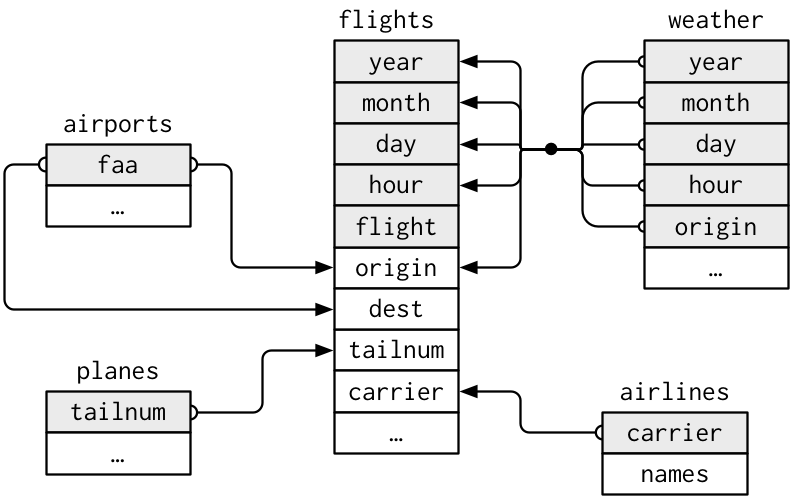

---

# Selecting rows using `filter`

``` r
filter(flights, month == 1 & day == 2)
```

```
## # A tibble: 943 × 19
##     year month   day dep_time sched_dep_time dep_delay arr_time sched_arr_time
##    <int> <int> <int>    <int>          <int>     <dbl>    <int>          <int>
##  1  2013     1     2       42           2359        43      518            442
##  2  2013     1     2      126           2250       156      233           2359
##  3  2013     1     2      458            500        -2      703            650
##  4  2013     1     2      512            515        -3      809            819
##  5  2013     1     2      535            540        -5      831            850
##  6  2013     1     2      536            529         7      840            828
##  7  2013     1     2      539            545        -6      959           1022
##  8  2013     1     2      554            600        -6      845            901
##  9  2013     1     2      554            600        -6      841            851
## 10  2013     1     2      554            600        -6      909            858
## # ℹ 933 more rows
## # ℹ 11 more variables: arr_delay <dbl>, carrier <chr>, flight <int>,
## #   tailnum <chr>, origin <chr>, dest <chr>, air_time <dbl>, distance <dbl>,
## #   hour <dbl>, minute <dbl>, time_hour <dttm>
```
]
.pull-right[
In pandas: simply indexing with condition!

``` python
flights = flights[ (flights.month == 1) 
                 & (fligths.day == 2) ]
```
]

---

# Filter and the `%in%` operator

``` r
sep_oct <- filter(flights, month %in% c(9, 10))
sep_oct
```

```
## # A tibble: 56,463 × 19
##     year month   day dep_time sched_dep_time dep_delay arr_time sched_arr_time
##    <int> <int> <int>    <int>          <int>     <dbl>    <int>          <int>
##  1  2013    10     1      447            500       -13      614            648
##  2  2013    10     1      522            517         5      735            757
##  3  2013    10     1      536            545        -9      809            855
##  4  2013    10     1      539            545        -6      801            827
##  5  2013    10     1      539            545        -6      917            933
##  6  2013    10     1      544            550        -6      912            932
##  7  2013    10     1      549            600       -11      653            716
##  8  2013    10     1      550            600       -10      648            700
##  9  2013    10     1      550            600       -10      649            659
## 10  2013    10     1      551            600        -9      727            730
## # ℹ 56,453 more rows
## # ℹ 11 more variables: arr_delay <dbl>, carrier <chr>, flight <int>,
## #   tailnum <chr>, origin <chr>, dest <chr>, air_time <dbl>, distance <dbl>,
## #   hour <dbl>, minute <dbl>, time_hour <dttm>
```

- In python: just `flights[ flights.month.isin([9, 10]) ]`

---

# Selecting columns using `select`

``` r
select(flights, year, month, day)
```

```
## # A tibble: 336,776 × 3
##     year month   day
##    <int> <int> <int>
##  1  2013     1     1
##  2  2013     1     1
##  3  2013     1     1
##  4  2013     1     1
##  5  2013     1     1
##  6  2013     1     1
##  7  2013     1     1
##  8  2013     1     1
##  9  2013     1     1
## 10  2013     1     1
## # ℹ 336,766 more rows
```
] 
.pull-right[
- Can match column names

``` r
select(flights, year, month, contains("delay"))
```

```
## # A tibble: 336,776 × 4
##     year month dep_delay arr_delay
##    <int> <int>     <dbl>     <dbl>
##  1  2013     1         2        11
##  2  2013     1         4        20
##  3  2013     1         2        33
##  4  2013     1        -1       -18
##  5  2013     1        -6       -25
##  6  2013     1        -4        12
##  7  2013     1        -5        19
##  8  2013     1        -3       -14
##  9  2013     1        -3        -8
## 10  2013     1        -2         8
## # ℹ 336,766 more rows
```
]

- In pandas: `flights[['year', 'month', 'day']]`

---

# Column ranges and `select`

``` r
select(flights, year:day, dest:hour)
```

```
## # A tibble: 336,776 × 7
##     year month   day dest  air_time distance  hour
##    <int> <int> <int> <chr>    <dbl>    <dbl> <dbl>
##  1  2013     1     1 IAH        227     1400     5
##  2  2013     1     1 IAH        227     1416     5
##  3  2013     1     1 MIA        160     1089     5
##  4  2013     1     1 BQN        183     1576     5
##  5  2013     1     1 ATL        116      762     6
##  6  2013     1     1 ORD        150      719     5
##  7  2013     1     1 FLL        158     1065     6
##  8  2013     1     1 IAD         53      229     6
##  9  2013     1     1 MCO        140      944     6
## 10  2013     1     1 ORD        138      733     6
## # ℹ 336,766 more rows
```
] 
--
.pull-right[
- Or exclude columns and ranges

``` r
select(flights, -year, -(dest:hour))
```

```
## # A tibble: 336,776 × 14
##    month   day dep_time sched_dep_time dep_delay arr_time sched_arr_time
##    <int> <int>    <int>          <int>     <dbl>    <int>          <int>
##  1     1     1      517            515         2      830            819
##  2     1     1      533            529         4      850            830
##  3     1     1      542            540         2      923            850
##  4     1     1      544            545        -1     1004           1022
##  5     1     1      554            600        -6      812            837
##  6     1     1      554            558        -4      740            728
##  7     1     1      555            600        -5      913            854
##  8     1     1      557            600        -3      709            723
##  9     1     1      557            600        -3      838            846
## 10     1     1      558            600        -2      753            745
## # ℹ 336,766 more rows
## # ℹ 7 more variables: arr_delay <dbl>, carrier <chr>, flight <int>,
## #   tailnum <chr>, origin <chr>, minute <dbl>, time_hour <dttm>
```
]
---

# `select()` helper functions

There are a number of helper functions you can use within `select()`:

- `starts_with("abc")`: matches names that begin with “abc”.

- `ends_with("xyz")`: matches names that end with “xyz”.

- `contains("ijk")`: matches names that contain “ijk”.

- `matches("(.)\\1")`: selects variables that match a regular expression.

- `num_range("x", 1:3)`: matches x1, x2 and x3.

In pandas: use the generic function `df.filter(regex='^abc')`

---

# Changing columns using `mutate`
.pull-left[
- `mutate()` can add or modify the columns in a data.frame

``` r
flights %>%
  mutate(
    gain = dep_delay - arr_delay,
    speed = distance / air_time * 60
  ) %>% 
  select(year:day, gain, speed)
```

```
## # A tibble: 336,776 × 5
##     year month   day  gain speed
##    <int> <int> <int> <dbl> <dbl>
##  1  2013     1     1    -9  370.
##  2  2013     1     1   -16  374.
##  3  2013     1     1   -31  408.
##  4  2013     1     1    17  517.
##  5  2013     1     1    19  394.
##  6  2013     1     1   -16  288.
##  7  2013     1     1   -24  404.
##  8  2013     1     1    11  259.
##  9  2013     1     1     5  405.
## 10  2013     1     1   -10  319.
## # ℹ 336,766 more rows
```
]
.pull-right[
- pandas are more wordy there:

``` python
flights['gain'] = flight['dep_delay'] 
                - flight['arr_delay']
flights['speed'] = flight['distance'] 
                 / flight['air_time'] * 60
flights = flights['year', 'month', 'day', 
                  'gain', 'speed']
```
]

---

# Some convenient but secondary functions

- `rename()` can change the name of a column

``` r
flights |> 
  rename(airline = carrier) |>
  names()
```

```
##  [1] "year"           "month"          "day"            "dep_time"      
##  [5] "sched_dep_time" "dep_delay"      "arr_time"       "sched_arr_time"
##  [9] "arr_delay"      "airline"        "flight"         "tailnum"       
## [13] "origin"         "dest"           "air_time"       "distance"      
## [17] "hour"           "minute"         "time_hour"
```
--

- `relocate()` can change the order of the columns

```r
# This will put `hour` and `distance` on the left:
flights |> 
  relocate(hour, distance)
```
- You can also use the `.before` and `.after` arguments to move columns

```r
flights |> 
  relocate(year:dep_time, .after = time_hour)
flights |> 
  relocate(starts_with("arr"), .before = dep_time)

```
---