Basic Interactions with R and Python

class: center, middle, inverse, title-slide

.title[
# Basic Interactions with R and Python
]
.subtitle[
## Variables, assignments, and functions
]
.author[
### Guillaume Falmagne
]
.date[
### <br> Sept. 9th, 2024
]

---

# What is R? What is Python?

.pull-left[
## .center[R]
- R is a programming language with a focus on **statistical computing and data visualization**

- Created in 1993

- Open source implementation of (derived from) the S-language from the mid-70s

- Very popular in academia, with over 17000 user-contributed **packages**
]
.pull-right[
## .center[Python]
- Python is a **general-purpose** programming language, focusing on **readability**

- Created in 1991

- One of the most popular languages, especially since the rise of **machine learning**

- General purpose = including scientific/academic/statistics problems 
]

---

# Why do we like them?

## R and Python
- **Open source**, cross platform, easy to learn, **concise** and readable

- Careful code can be reasonably fast

- Easy interaction/**interface with faster languages** like C++ (and FORTRAN)

- Accommodates **several programmings paradigms** (though R is not great at object-oriented programming)

- Large helpful **online community**

.pull-left[
## .center[R]
- strong focus on data exploration + high quality plotting libraries 
- 17,000 packages = very high probability that the analysis
you want is already implemented.
]
.pull-right[
## .center[Python]
- There are great modules in all domains, not only plotting or statistics
]

---

class: left, top
background-image: url(figures/slowpython.jpg)
background-position: center right
background-size:  30%

# Why do we hate it?

- **Typical code is very slow**  
... but can be more than **compensated by using appropriate modules**  
implemented in more efficient languages (typically C++)

### R 
- Not really suited for general purposes (while Python is!), but people push it

- Check R-Inferno for all the traps in R

![:scale 17%](figures/R_inferno.jpg)

---

class: left, top
background-image: url(figures/offandon.jpg)
background-position: center right
background-size:  33%

# A few practical things to know

### R and Python
- **case-sensitive**

- **dynamically-typed**: no need to specify the type of a variable when it is defined  
(it "automatically" determines its type from the input content),  
whereas necessary in e.g. C++

### Python
- **Indentation** is used as key syntax (e.g. embedded loops)

### *All* languages
- Environment variables, stuck processes, conflicting commands, cache,  
broken untested situation...  
**Turning off and on again** can often solve mysterious error messages,   
especially for introductory steps!

---

# Modules / packages / namespace

How to use functions that are *not from the "core" language* and not within your main script?  
**Namespace** = set of names of functions/object/... from an module or package

.pull-left[
### R
- Functions from installed packages can be called **without reference** to the package namespace. But this can lead to **conflicts** (one function name used in two packages)

``` r
library(DescTools)
a <- c(1,2,2,3)
Mode(a)
# also works, and safer for namespace
 `DescTools::`Mode(a)
```
]
.pull-right[
### Python
- **"modules"** must be imported to use the associated functionalities. Must specify that functions are from that module.
```python
import numpy as `np`
import scipy as `sc`
a = `np`.array([1,2,2,3])
mode = `sc`.stats.mode(a)
```
]

---

class: left, top
background-image: url(figures/rstudio-panes-labeled.jpeg)
background-position: center
background-size:  65%

# Rstudio

---

class: left, top
background-image: url(figures/VsCode.png)
background-position: center
background-size:  83%

# VsCode

---

# Arithmetics and math functions

.pull-left[
### R

``` r
# This is a comment, 
# which is ignored by R because it's after the #  
1 + 3**2
```

```
## [1] 10
```

``` r
sin(0.4) * log(15) + exp(3) / atan(27)
```

```
## [1] 14.15005
```
]
.pull-right[
### Python

``` python
# Same comment syntax in Python
1 + 3**2
```

```
## 10
```

``` python
import math as m
m.sin(0.4) * m.log(15) + m.exp(3) / m.atan(27)
```

```
## 14.150045221228968
```
]

---

# Assigning Variables

.pull-left[
### R

Variables can be assigned using the assignment operator `<-` or `=`

``` r
x <- 10
y = 5
```

Typing a variable's name will show its contents:

``` r
x
```

```
## [1] 10
```

The [1] in the output refers to the position in the vector (here, a scalar) 
]
.pull-right[
### Python

Assignment only with `=`

```python
x = 10
y = 5
```
Same in Python console

``` python
x = 10
x
```

```
## 10
```
]

---

# Vectors and arrays

.pull-left[
### R

- Vectors are the main data structure in R
- All objects in a vector are of the same type  
(logical, integer, double, character, ...)
- Single variables are length-one vectors

``` r
# Concatenate function
x <- c(1, 2, 3, 4) 
y <- c("a", "b", "c", "d")

# Sequences
one_to_four <- 1:4

# seq function 
one_to_four <- seq(1, 4, by = 1)

# rep function 
one_four_times <- rep(1, 4)
```
]
.pull-right[
### Python

- **numpy** is key for arrays
- All objects in an array are of the same type  
(bool, float, ...)

```python
import numpy as np

x = np.array( [1, 2, 3, 4] )
# simple lists are better for strings in python
y = ["a", "b", "c", "d"]

# List and array versions exist
one_to_four = list(range(1, 4))
one_to_four = np.arange(1, 4)

one_to_four = np.arange(1, 5, 1)

one_four_times = np.full(4, 1)
```
]

---

# Indexing objects

- Values inside an object can be accessed by the bracket `[]` operator
- **Indexing starts at 0 in Python (vs 1 in R)**. This means the last element of `range(0, n)` is `n-1`

.pull-left[
### R

``` r
x = 1:6
x[2]    # Indexing a single value
```

```
## [1] 2
```

``` r
x[1:3] # Indexing using a vector
```

```
## [1] 1 2 3
```

``` r
x<4
```

```
## [1]  TRUE  TRUE  TRUE FALSE FALSE FALSE
```

``` r
x[x<4] # Indexing using a logical condition
```

```
## [1] 1 2 3
```
]
.pull-right[
### Python

``` python
import numpy as np
x = np.arange(1, 7)
x[1]
```

```
## 2
```

``` python
x[0:3]
```

```
## array([1, 2, 3])
```

``` python
x<4
```

```
## array([ True,  True,  True, False, False, False])
```

```python
x[x<4]
```
]

---

# Lists

- Lists are a vector of references to variables of any kind

.pull-left[

### R

``` r
l1 <- list(1, 2, 3)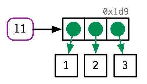
```

![:scale 40%](figures/list.png)

``` r
l1[[2]] <- "a"
l1
```

```
## [[1]]
## [1] 1
## 
## [[2]]
## [1] "a"
## 
## [[3]]
## [1] 3
```
]
.pull-right[
### Python

- Lists are the basic object of Python.  
- Extremely versatile and allows magic syntax (list comprehension).  
- But can be very slow!

``` python
l1 = [1, 'a', 3]
l2 = [2*i for i in l1]
l2
```

```
## [2, 'aa', 6]
```
]

---

# R: A variable name and its contents

.pull-left[

``` r
x <- c(1, 2, 3)
x
```

```
## [1] 1 2 3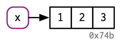
```

![:scale 40%](figures/x_address.png)

```r
y <- x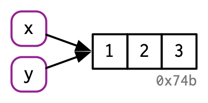
```
![:scale 40%](figures/binding-2.png)
]
.pull-right[

- Copy on modify

``` r
x <- c(1, 2, 3)
y <- x

y[[3]] <- 4
x
```

```
## [1] 1 2 3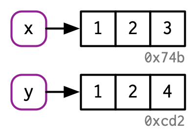
```
![:scale 40%](figures/binding-3.png)

]

---

# Python: variables are references!

``` python
i = 5     # create int(5) instance, bind it to i
j = i     # bind j to the same int as i
j = 2     # create int(3) instance, bind it to j
i         # i still bound to the int(5), j bound to the int(3)
```

```
## 5
```

Lists, as integers, are objects that are "referenced" (i.e. pointed to) by variable names

``` python
i = [1,2,3]   # create the list instance, and bind it to i
j = i         # bind j to the same list as i
i[0] = 4      # change the first item of i
j             # j is still bound to the same list as i
```

```
## [4, 2, 3]
```

Those are **not bugs, but features**... They become bugs if you are not aware of how mutability works for your object!

---

# Special values in R: `NA` and `NULL`

.pull-left[
- `NA` stands for "Not Available".
- Used to represent missing values in R.
- Can have a class (like `NA_real_`, `NA_integer_`).

``` r
# Vector with NA values
data_vector <- c(1, 2, NA, 4, 5)

# Sum function with NA
sum(data_vector) # This will return NA
```

[1] NA

``` r
# Handling NA values
sum(data_vector, na.rm = TRUE) 
```

[1] 12

- There is an equivalent of `NA` in `pandas`   
(extension of numpy)
- It is usually `np.nan` (not-a-number), also used for `/0`
]
.pull-right[
- `NULL ` represents the absence of a value or an undefined value. It's different than NA. 
- While NA represents missingness, NULL indicates the absence of a structure.
- NULL can be output when the result is undefined.

``` r
# Length of NA and NULL
length(NA)    # Returns 1
```

```
## [1] 1
```

``` r
length(NULL)  # Returns 0
```

```
## [1] 0
```

- The equivalent of `NULL` in Python is `None`
]
---

# Arithmetics on vectors

Basic arithmetic operations can be performed on variables.

.pull-left[

### R

``` r
x = c(1, 3)
y = c(2, 5)
Sum <- x + y
Sum
```

```
## [1] 3 8
```

``` r
product <- x * y
product
```

```
## [1]  2 15
```

]
.pull-right[
### Python

``` python
import numpy as np
x = np.array([1,3])
y = np.array([2,5])
Sum = x+y
Sum
```

```
## array([3, 8])
```

``` python
product = x * y
product
```

```
## array([ 2, 15])
```
]

---

# Vectorized operations

.left-column60[
### R

``` r
x <- seq(1, 13, length.out = 5)
x
```

```
## [1]  1  4  7 10 13
```

``` r
x + 1
```

```
## [1]  2  5  8 11 14
```

``` r
sqrt(x)
```

```
## [1] 1.000000 2.000000 2.645751 3.162278 3.605551
```

### Python
Vectorized operations are extremely faster than for loops! Try this:
```
x = np.arange(0,100000) 
np.sqrt(x)
[sqrt(x) for i in x] # extremely slower!
```
]
.right-column60[
![:scale 100%](figures/forloopsnumpy.png)
]

---

# Matrices

.pull-left[

### R

- Matrices are like vectors but with two dimensions

``` r
mat = matrix(1:12, nrow = 4, ncol = 3)
mat
```

```
##      [,1] [,2] [,3]
## [1,]    1    5    9
## [2,]    2    6   10
## [3,]    3    7   11
## [4,]    4    8   12
```

- We index matrices using a comma [rows, columns]

``` r
mat[1,2]
```

```
## [1] 5
```
]
.pull-right[
### Python
- This is where numpy starts to show its power
- Can have arbitrary number of dimensions

``` python
import numpy as np
mat = np.arange(1, 13).reshape((4, 3), order='F')
mat
```

```
## array([[ 1,  5,  9],
##        [ 2,  6, 10],
##        [ 3,  7, 11],
##        [ 4,  8, 12]])
```

``` python
mat[0,1]
```

```
## 5
```

``` python
mat4 = np.ones((3,3,3,3)) # 4-dim matrix of 1's
```
]

---

# Matrices

.pull-left[

### R
We can check the shape a matrix using dim()

``` r
dim(mat)
```

```
## [1] 4 3
```

We can access full rows or columns by ommiting one index

``` r
mat[1,] # First row 
```

```
## [1] 1 5 9
```

``` r
mat[,1] # First column 
```

```
## [1] 1 2 3 4
```
]
.pull-right[
### Python

``` python
mat.shape
```

```
## (4, 3)
```

``` python
mat[0, :] # First row
```

```
## array([1, 5, 9])
```

``` python
mat[:, 0] # First column 
```

```
## array([1, 2, 3, 4])
```
]

---

# Vectors and matrices are homogeneous

- All the elements in an atomic vector or matrix (R) or array (Python) must be of the same type

.pull-left[
### R

``` r
(num_x = rnorm(3))
```

```
## [1]  1.9849356 -0.9247631 -1.7900920
```

``` r
(char_y = letters[1:3])
```

```
## [1] "a" "b" "c"
```

``` r
(logic_z = num_x > 0)
```

```
## [1]  TRUE FALSE FALSE
```

### Python
Can define type in numpy arrays

``` python
floatarray = np.arange(5, dtype=float)
```
]
.pull-right[
![:scale 65%](figures/summary-tree-atomic.png)
]

---

# R: auto-conversion of types

``` r
num_x[4] <- "a"
num_x
```

```
## [1] "1.98493560452221"   "-0.924763141709784" "-1.79009195048663" 
## [4] "a"
```

- This can cause subtle bugs:

```r
num_x + 1
```
Error in `num_x + 1`:  
! non-numeric argument to binary operator

This is **impossible with numpy** (immutable type), but possible with Python lists

---

# R: Factor vectors

- A factor is a data type used in R for categorical variables.
- Kind of cross between numeric and character
- Internally, R stores factors as integers and maintains a level set for factor values.
- Designed to handle categorical data, especially in the context of linear models
  - Things like: Color, Species, Batch, Sex, Treatment-Control, ...
- Has a fixed number of possible values

``` r
# Create a sample vector
color_vector <- c("Red", "Blue", "Green", "Red", "Blue")

# Convert the vector to factor type
color_factor <- factor(color_vector)

# Display the factor
color_factor
```

```
## [1] Red   Blue  Green Red   Blue 
## Levels: Blue Green Red
```

- Equivalent in Python, with `pandas`: `s = pandas.Series(["a","b","c","a"], dtype="category")`

---
# Python: dictionaries

- Dictionaries are extremely practical for any **book-keeping** task
- They **match pairs of values** of any type. Keys and values are **not** ordered.

``` python
dicto = {'first': 1, 'second': 2.0, 'my_third_object': 'not_an_int'}
dicto.keys()
```

```
## dict_keys(['first', 'second', 'my_third_object'])
```

``` python
dicto.values()
```

```
## dict_values([1, 2.0, 'not_an_int'])
```

``` python
dicto['second']
```

```
## 2.0
```

``` python
dicto['first'] = [1, 5, 7]
```

---

# R: Names attributes

.pull-left[
- Vectors, matrices, list, and other objects can have names associated with their contents.

- You can name a vector in three ways:

``` r
# When creating it: 
x <- c(a = 1, b = 2, c = 3)

# By assigning a character vector to names()
x <- 1:3
names(x) <- c("a", "b", "c")

# Inline, with setNames():
x <- setNames(1:3, c("a", "b", "c"))
x
```

```
## a b c 
## 1 2 3
```
]
.pull-right[
![:scale 60%](figures/attr-names-1.png)

![:scale 30%](figures/attr-names-2.png)

- In Python, would need to use dictionaries for this functionality, but not recommended for numerical computations.  
`dataframe` in `pandas` can get names for columns.
]

---

# Objects can be indexed by their names

.pull-left[
- Vectors

``` r
x <- c(a = 1, b = 2, c = 3)
x["a"] # single brackets give you a list or vector
```

```
## a 
## 1
```

``` r
x[c("c", "b")]
```

```
## c b 
## 3 2
```
]
.pull-right[
- Lists

``` r
l <- list(a = 1, b = 2, c = 3)
l[["a"]] # double brackets give you a single element
```

```
## [1] 1
```

``` r
l[c("c", "b")]
```

```
## $c
## [1] 3
## 
## $b
## [1] 2
```

]
---

# R: Dataframes

.pull-left[

- The secret sauce of R for biology

- Basically a list of vectors of the same length

- Each column is an atomic vector of a given type

``` r
d1 <- data.frame(x = c(1, 5, 6), 
                 y = c(2, 4, 3), 
                 id = c("a", "b", "c"))
d1
```

```
##   x y id
## 1 1 2  a
## 2 5 4  b
## 3 6 3  c
```

``` r
names(d1)
```

```
## [1] "x"  "y"  "id"
```
]
.pull-right[
- Dataframes have 2 attributes:
    - rownames (don't use these)
    - names (column names)

```r
df = data.frame(x = 1:3,
                y = letters[1:3])
```
![:scale 60%](figures/data-frame-1.png)
]

---

# R: Dataframe columns

- Data frame colums can also be indexed using the `$` operator
- This operator can also create new columns

.pull-left[

``` r
d1
```

```
##   x y id
## 1 1 2  a
## 2 5 4  b
## 3 6 3  c
```

``` r
d1$x
```

```
## [1] 1 5 6
```

``` r
d1$sum <- d1$x + d1$y
d1$sum
```

```
## [1] 3 9 9
```
]

.pull-right[

- We can also use `$` to erase columns

``` r
d1
```

```
##   x y id sum
## 1 1 2  a   3
## 2 5 4  b   9
## 3 6 3  c   9
```

``` r
d1$sum <- NULL
d1
```

```
##   x y id
## 1 1 2  a
## 2 5 4  b
## 3 6 3  c
```
]

---
# Python: pandas dataframes

.left-column60[
- Very similar functions than R dataframes
- `pandas` has enormous amounts of useful functionalities 
- Equivalent of `rownames`: `df.index`

``` python
import pandas as pd 
data = { # dictionaries is only one of the initialisation methods
        'x' : [1, 5, 6], 
        'y' : [2, 4, 3], 
        'id' : ['a', 'b', 'c'], 
        }
#load data into a DataFrame object:
df = pd.DataFrame(data)
print(df)
```

```
##    x  y id
## 0  1  2  a
## 1  5  4  b
## 2  6  3  c
```
]
.right-column60[
- Can access row and columns,  
both returning a `Series` object, equivalent of `numpy` array

``` python
df.loc[0] # row access.  
```

```
## x     1
## y     2
## id    a
## Name: 0, dtype: object
```

``` python
df['id'] # column access.
```

```
## 0    a
## 1    b
## 2    c
## Name: id, dtype: object
```
]
---

# R: With and within

.pull-left[
- `with()` function

- Used to evaluate expressions in the context of a specific dataset.
- Helps to reduce text redundancy when referring to data frame columns.

``` r
df <- data.frame(
  x = rnorm(5),
  y = runif(5)
)
sum(df$x + df$y)
```

[1] 4.923928

``` r
with(df, sum(x + y))
```

[1] 4.923928
]

.pull-right[
- `within()` function

- Used to modify data frames or lists.
- Evaluates expressions inside the data frame, making it easier to create or modify columns.

``` r
# Modify df using within
df_modified <- within(df, {
  z = x + y
  w = x * 2
})
df_modified
```

```
##             x         y          w          z
## 1  0.28439727 0.9486180  0.5687945  1.2330152
## 2 -0.05483241 0.3728396 -0.1096648  0.3180072
## 3  0.42646721 0.7197441  0.8529344  1.1462113
## 4 -0.77004584 0.6154574 -1.5400917 -0.1545884
## 5  1.54800866 0.8332741  3.0960173  2.3812827
```
]

---
# Functions (in R)

.pull-left[
- Functions are pieces of code producing some output from some set of arguments

- Allows us to repeat the same procedure several times with different inputs without repeating code, so it improves conciseness and readability

- Packages are mostly just groups of related functions (and classes)

- The help() function shows the help page for any function

```r
help(apply)
?apply
```

]
.pull-right[

- Arguments can be used to alter a function's behavior

``` r
input = c(3, 4, 7, 7, 8, NA)
mean(x = input)
```

```
## [1] NA
```

- We can deal with `NA` with another argument of the mean:

``` r
mean(x = input, na.rm = TRUE)
```

```
## [1] 5.8
```
]

---

# Creating Functions

.pull-left[
### R
Functions can be defined using the `function()` keyword.

``` r
multiply <- function(a, b) {
  result <- a * b
  return(result)
}
multiply
```

```
## function(a, b) {
##   result <- a * b
##   return(result)
## }
```

``` r
multiply(3, 2)
```

```
## [1] 6
```
]
.pull-right[
### Python

``` python
def multiply(a, b):
  return a * b
multiply
```

```
## <function multiply at 0x714ea3f0d510>
```

``` python
multiply(3, 2)
```

```
## 6
```
]

---

# Loading Packages

.pull-left[
To load packages in R, use the `library()` function.

```r
library(dplyr)
library(ggplot2)
```

To install a missing package, use the `install.packages()` function

```r
# notice the quotation marks!!
install.packages("ggplot2") 
```

Also, take a look at the `pak` package:

- [https://github.com/r-lib/pak](https://github.com/r-lib/pak)

```r
pak::pkg_install("ggplot2")
```
]
.pull-right[
![:scale 100%](figures/libraries.webp)
]

---

# Working Directory

To check the current working directory, use `getwd()`.

```r
current_dir <- getwd()
```

To set the working directory, use `setwd()`.

```r
setwd("/path/to/directory")
```

**Using Rstudio or vscode projects takes care of this for you.**